Study of heat transfer coefficient in helical coil (0)

INSTITUTO POLITECNICO DO PORTO
INSTITUTO SUPERIOR DE ENGENHARIA DO PORTO
CHEMICAL ENGINEERING DEPARTMENT
PORTUGAL
Marvin Üürike
Tallinn University of Technology
Faculty of Chemical and Materials Technology
Department of Chemical Engineering
Estonia
ERASMUS PROJECT
STUDY OF THE HEAT TRANSFER COEFFICIENT IN A HELICAL COIL
Supervisor: Albina Ribeiro
Porto 2015
Abstract
The following work investigates overall heat transfer coefficient of a helical coil and how it changes in different situations. The variables investigated were flow rate inside a submerged helical coil and agitation of the bath .
To investigate the change in heat transfer coefficient in different situations, a simple experiment was set up. It consisted of a rectangular isolated tank , which was filled with water, submerged steel coil and an agitator. A rotameter was used to measure the flow rate, and a pump was used to force the water through the coil. A thermocouple was placed at each end of the coil to measure the inlet and outlet temperatures and another thermometer used to measure the overall temperature of the water inside the bath.
Two different approaches were taken, one of them was investigating heat change coefficient in steady state and the other was studying it in an unsteady state. In steady state, a constant flow rate and agitation was applied until temperatures stayed constant, then were the readings taken. In unsteady state, bath was heated up and then cooled down with cold water running through the submerged coil and temperature readings were taken every five minutes.
A theoretical overall heat transfer coefficient was calculated using different sources of literature and then they were compared to experimental coefficients . The difference is explained based on the conditions of equations and experimental setup.
The results showed that overall heat transfer coefficient changed as expected , it was bigger with higher flow rates, which directly results in higher Reynolds numbers , and higher agitation rates. Some anomalies did occur , but they can be explained with atypical details in experimental setup.

Table of Contents

Table of Contents 5
1Introduction 1
2Experimental description 12
2.1Experimental apparatus 12
2.2Experimental procedure 14
2.2.1Steady state experiments 14
2.2.2Unsteady state experiments 15
3Results and discussion 16
3.1Steady state 16
3.2Unsteady state 22
3.3Theoretical 28
4Conclusions and suggestions for future work 32
5Bibliography 34
APPENDICES 31
A.1 Calibration of the rotameter 31
A .2Calibration of Thermocouple and Electronic thermometer 32
A.3 Calculation example 34
1 Introduction 1
2 Experimental description 12
2.1 Experimental apparatus 12
2.2 Experimental procedure 13
2.2.1 Steady state experiments 13
2.2.2 Unsteady state experiments 13
3 Results and discussion 14
3.1 Steady state 14
3.2 Unsteady state 20
3.3 Theoretical 25
4 Conclusions and suggestions for future work 28
5 Bibliography 29
APPENDICES 30
A.1 Calibration of the rotameter 30
A.2Calibration of Thermocouple and Electronic thermometer 31
A.3 Calculation example 33
List of figures
Figure 1, Types of agitators ( http://www.thermopedia.com/content/1176/ 9
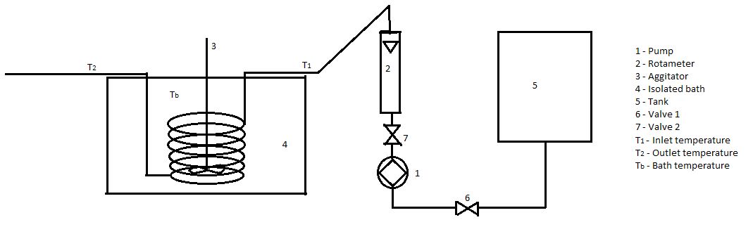
Figure 2: Schematic diagram of the apparatus 12
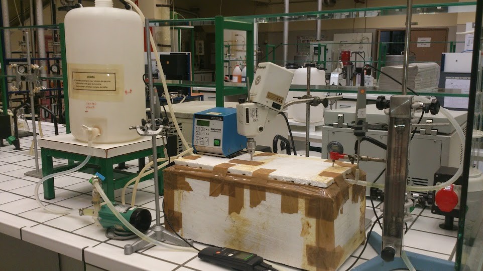
Figure 3: Picture of the experimental setup 13
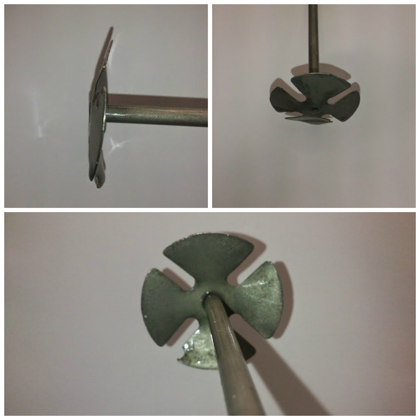
Figure 4: Picture of the agitator blade 14
Figure 5: Steady state U with the bath temperature approximately 33C 16
Figure 6: Steady state U with the bath temperature approximately 44C 18
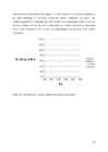
Figure 7: Comparison of steady coefficient of different state heat transfer bath temperatures at 618 rpm. 20
Figure 8: Comparison of steady state heat transfer coefficient of different bath temperatures at 1703 rpm. 21
Figure 9: Unsteady state U considering no heat loss 22
Figure 10: Bath heat loss 23
Figure 11: Unsteady state U considering heat loss 24
Figure 12: Comparison of steady state and unsteady state heat transfer coefficient at agitations of 618 rpm and 1703 rpm. 26
Figure 13: Theoretical heat transfer coefficient according to Richardson and Coulson 28
Figure 14: Theoretical heat transfer coefficient according to Geankoplis. 29
Figure 15: Calibration curve for the rotameter 31
Figure 16: Calibration curve for the outlet (T1) thermocouple. 32
Figure 17: Calibration curve for the inlet (T2) thermocouple. 33
Figure 18: Calibration curve for electronic thermometer 33
List of Symbols
A
Heat exchange area
m2
Ai
Inside surface area coil
m2
Ao
Outside surface area coil
m2
cp
Specific heat
J•kg-1•K-1
cpa
Specific heat of the water inside the bath
J•kg-1•K-1
cpb
Specific heat of the water inside the coil
J•kg-1•K-1
deq
Equivalent diameter of the tank
m
da
Diameter of the agitator
m
dc
Diameter of the coil
m
din
Inside diameter of the tube
m
hi
Convective heat transfer coefficient inside the coil
W•m-2•K-1
ho
Convective heat transfer coefficient outside coil
W•m-2•K-1
k
Slope of linear function
k
Thermal conductivity
W•m-1•K-1
Mass flow
kg•s-1
ma
Mass of water inside the bath
kg
Mass flow rate inside the coil
kg•s-1
Nu
Nusselt number
q
Heat
J
Q
Heat transfer rate
J•s-1
U
Heat transfer coefficient
W•m-2•K-1
ΔT
Temperature difference
K
ΔTlm
Log mean temperature difference
K
Δx
Thickness of coil wall
m
lv
Length of the square bath side
m
L
Length of the agitator blade
m
N
Agitator speed
rps
μ
Viscosity of water at wall temperature
Pa·s
μ
Viscosity of water
Pa·s
k
Thermal conductivity of water in the bath
W•m-1•K-1
dg
Distance between two spirals
m
cp
Heat capacity of water
J•kg-1•K-1
dp
Height of the coil
m
W
Height of the blades of the agitator
m
do
Outside diameter of the tube
m

Introduction

Heat transfer is a very common phenomenon in chemical engineering. Heat exchangers are one of the most common technological devices used in different areas of chemical industries. There are a large number of options available for the exchange of thermal power . The choice usually comes down to different factors, in which the heat exchanger must be performing. One of the most common heat exchangers structure is the tubular form. In the field of tubular heat exchangers, one way is to bend the tube helicoidally, which makes the tube a lot more compact and less expensive, because less material is needed to jacket the tube. Due to the increased number of turns of the helix , additional turbulence is generated inside the tube and therefore the heat transfer coefficient of the helical coil is larger that of the corresponding straight tube. In chemical industries there are many applications, which use coils as heat exchangers such as in small nonindustrial boiler systems where water is heated up or steam is generated inside the helical coil by direct heating via burning fuel such as diesel oil or other burning materials. Polyethylene is also manufactured inside helical coils, where oxidation of ethylene takes place . The heat from this exothermic reaction is taken away by cooling water circulating around the helical coils. In many industrial applications helical coils are used to heat up cold liquid circulating around the coils, by steam condensation inside the coil. In addition to heating up the liquid around, coils can also be used to cool it down, if the bulk liquid around the coil acts as a reactor and the reaction is exothermic. There are many applications for helical coils that have been used in chemical industries for several decades. (Hewitt, et al., 1994)
The three basic mechanisms in heat transfer are conduction, convection and radiation . In chemical engineering conduction and convection are the mechanisms, which are applied most commonly . When talking about conduction, the heat can be transferred through gases, liquids or solids. The heat is transferred by the energy of motion adjacent molecules. The molecules with higher energy and motion affect adjacent molecules with lower energy and motion, imparting them energy. In conduction energy can be transferred by free electrons, which play a big role in heat transfer in metals. Convection stands for heat transferring through gases and liquids with bulk movements of them, or the mixing of macroscopic elements of hotter portions with cooler portions of liquid or gas. It also often involves a solid surface. It should be noted that there is a difference between forced convection and natural convection. In forced convection the fluid or gas is forced to flow over a solid surface with a fan or pump. In natural convection, the motion of molecules in gas or liquid is not forced, but natural. Radiation differs from conduction and convection in that manner , that it does not need any physical medium for its propagation. Radiation is the transfer of energy through space by means of electronic waves. It is similar how electromagnetic light waves transfer light, which also means that the same laws apply . The most common example to characterize radiation is the way heat is transferred to Earth from the Sun. (Geankoplis, 1993)
To be able to quantify the amount of heat exchanged with different heat transfer mechanisms or with all of them combined, many coefficients have developed according to characterize different material’s ability to exchange heat.
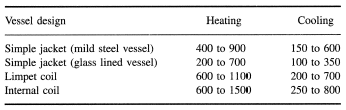
Fletcher has given some representative data on overall heat transfer coefficients that may be seen in agitated vessels. The range of these data shown in Table 1, illustrates some of the differences in heat transfer rates that may be experienced when using different types of heat exchangers. (Fletcher, 1987)
To calculate the amount of heat transferred, two different approaches must be taken depending on the nature of the heat transfer. Steady state and unsteady state heat transfers have to be calculated differently, because steady state heat transfer rate as the name suggests does not change in time, whereas the unsteady state heat transfer rate does.
Table 1: Overall heat transfer coefficients for heat transfer systems with coils or jackets. (Fletcher, 1987)
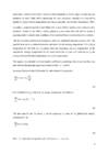
Consider a system consisting of a thermostatic bath with a coil immersed inside it and if the bath is maintained at a constant temperature and a cold liquid flows inside the coil, the global heat transfer coefficient is calculated using equations (1) and (2):
(0)
Where,
Q – Heat transfer rate, J•s-1
A – Heat exchange area, m2
ΔTlm – log mean temperature difference, K
Heat transfer rate can be calculated from the equation (2), where the specific heat is assumed to be constant and chosen for the mean temperature of the inlet and outlet temperatures of the coil.
(0)
Where,
– Mass flow, kg•s-1
cp – specific heat, J•kg-1•K-1
ΔT – temperature difference between the outlet and inlet temperatures of the fluid inside the coil, K
The unsteady state is a little more difficult to understand , because the temperatures are changing with time. The unsteady heat transfer is important because of the vast amount of heating and cooling problems occurring industrially. In metallurgical processes it is needed to predict the heating or cooling rates of various geometries of metals in order to know how much time it will take for them to reach a certain temperature. In the paper industry logs are immersed in steam baths before processing . In many processes materials are immersed in liquids of higher or lower temperatures resulting in unsteady heat transfer. (Geankoplis, 1993)
Consider a system formed by a tank filled with a mass of fluid inside which a helical coil is immersed. Inside the coil flows a cooling liquid at a given mass flow rate and the system is operating under unsteady state conditions. It is considered there is no heat loss to the exterior.
The heat transfer coefficient in an unsteady state was calculated using the equation (15). The specific heats were considered constants and chosen for the average temperature. The average temperature for the bath was calculated from the beginning and end temperatures of the experiment. Average temperature for the water inside the coil was calculated by taking the average between the inlet temperatures and outlet temperatures.
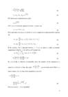
The equation to calculate the heat transfer coefficient considering there is no heat loss was derived from the principle equations in heat transfer (3, 4, and 5).
An energy balance to the fluid inside the bath at instant t is given by:
(0)
For the fluid flowing in the coil, the energy balance can be written as:
(0)
The heat transfer rate for instant t can be expressed in terms of the global heat transfer coefficient, U, by:
(0)
When the right sides of equations (4) and (5) are set to be equal.
(0)
(0)
If U and cpb are considered constant, then:
(0)
Which when inserted into equation (7) results in equation (9)
(0)
If the right sides of equations (3) and (4) are set to be equal with a replacement from equation (9)
(0)
(0)
If the equation (11) is integrated between t = 0 and an instant t, which corresponds temperatures of the fluid in the bath Tain and Ta respectively
(0)
(0)
If a set of data is obtained experimentally, where the variation of the temperatures is registered as a function of time, then a plot
against t can be made. If there is a linear variation, then the slope of the straight line is given by:
(0)
From the equation (14) U is calculated:
(0)
Where,
mb – mass flow rate of water inside coil, kg•s-1
cpb – specific heat of water inside coil, J•kg-1•K-1
C – slope of the linear function
ma – mass of water in bath, kg
cpa – specific heat of water in bath, J•kg-1•K-1
A – heat exchange area, m2
Considering that the thermal system under study is not well insulated and there was a heat loss, a second approach to calculate the global heat transfer coefficient can be taken. For each instant, t, the heat transfer rate received by the fluid flowing inside the coil can be calculated by:
(0)
Where,
- mass flow rate, kg.s-1
cp – specific heat of water inside coil at mean temperature, J•kg-1•K-1
∆T - temperature differences at inlet and outlet of the coil, K
(0)
Where,
Q – heat transfer rate, W
A – heat transfer area, m2
U – overall heat transfer coefficient, W•m-2•K-1
∆Tlm – log mean temperature difference, K
If a graphical plot of Q against A·∆Tlm is made and if a linear relation between the two variables is verified, then the average global heat transfer coefficient corresponds to the slope of the line. It is considered that the U does not vary with time.
Prediction of the overall heat transfer coefficient
In a tubular heat exchanger where the mechanisms of heat transfer involved are conduction and convection, the overall heat transfer coefficient can be predicted by the following equation.
(0)
Where,
hi – convective heat transfer coefficient inside the coil, W•m-2•K-1
ho – convective heat transfer coefficient outside the coil, W•m-2•K-1
Δx – thickness of the coil wall, m2
k – thermal conductivity of the steel coil, W•m-1•K-1
Ao – surface area outside the coil, m2
Ai – surface area inside the coil, m2
To determine if the flow pattern inside the coil was laminar or turbulent, a critical Reynolds number was calculated. When the Reynolds number is less than the critical Reynolds number, the flow pattern is laminar, and if the Reynolds number is greater than the critical Reynolds number, the flow pattern is turbulent. The critical Reynolds number is determined with the following equation (19). (Hewitt, et al., 1994)
(0)
For laminar flow inside straight tubes, the heat transfer coefficient can be predicted by. (Geankoplis, 1993):
(0)
Where,
k – thermal conductivity of the water, W•m-1•K-1
din – inner diameter of the tube, m
Heat transfer through tubes is well known and studied. Coils are very similar to tubes; expect that there is additional turbulence created in the liquid by the circular motion of the flow. Therefore it is usual to apply a correction for the inside coil heat transfer coefficient when compared to straight pipe . Hewitt et al. (1994) recommends the application of the equation (21).
(0)
Where,
din – inner diameter of the tube, m
dc – diameter of the coil, m
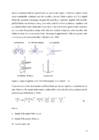
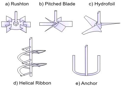
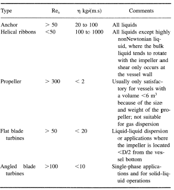
The heat transfer coefficient on the outside of the coil depends strongly on the rate of agitation and the type of agitator used. There are many types of agitators. They can be divided into five distinctly different agitator types, as seen on the Figure 1. A Rushton, turbine which cause considerable turbulence near the impeller, a pitched blade impeller with flat, angled blades that generates a diverging but generally axial flow, a hydrofoil impeller with carefully profiled blades that develop a strong , more truly, axial flow of low turbulence. Impellers such as a helical ribbon with a blade that moves close to the wall to force good overall circulation and an anchor that produces strong swirl with poor vertical mixing even when installed with baffles are used with more viscous fluids. The range of application for different agitators with a comment can be seen on the table 3. (Hewitt, et al., 1994)
Figure 1, Types of agitators ( http://www.thermopedia.com/content/1176/
To preview the outside heat transfer coefficient there are various empirical correlations in the open literature. For square tanks using a simple paddle stirrer the following equations can be used (Coulson & Richardson, 2004):
(0)
Where:
lv – length of the square bath side, m
L – length of the agitator blade, m
N – agitator speed, rps
μ – viscosity of water, Pa·s
k – thermal conductivity of water in the bath, W•m-1•K-1
dg – distance between two spirals, m
cp – heat capacity of water, J•kg-1•K-1
dp – height of the coil, m
W – height of the blades of the agitator, m
do – outside diameter of the tube, m
Table 2 - The range of application of agitators. (Hewitt et al, 1994)
Another correlation to calculate the outside convection heat transfer coefficient and which is valid for paddle agitators and circular tanks with no baffles is (Geankoplis, 1993):
(0)
deq - equivalent diameter of the tank, m
da – diameter of the agitator, m
μw – viscosity at wall temperature, Pas

Experimental description

Experimental apparatus

The experiments were carried out in the experimental apparatus, whose schematic diagram is shown in Figure 2.
Figure 2: Schematic diagram of the apparatus
The water used to flow through the steel coil was held in a reservoir, with a capacity of approximately 25 liters. A centrifugal pump was used to circulate the water from the tank to the coil and then to the drain. The flow rate of the water was measured using a calibrated rotameter. The coil was located inside the hot water rectangular bath with dimensions of 45,5 X 21,1 cm with no baffles. The height of the coil was 6,2 cm, the diameter of helix was 17,4 cm, the length of the tube in spiral was 4,72 m, and the internal diameter of the tube was 7,3mm and external diameter 1,1cm. The bath was heated with a Bioblock Scientific polystat microprocessor controlled electrical resistance . The agitation system was composed by a propeller fitted to a Heidloph Type RZR1 mixer. The speed of the agitator could be changed with the speed reducing controller. The temperature of the bath was measured with a simple Micro- tech electronic thermometer. The inlet and outlet temperatures of the water flowing inside the coil were measured with a calibrated thermocouples K type, which were linked to Testo 922 device .
Figure 3: Picture of the experimental setup
Figure 4: Picture of the agitator blade

Experimental procedure

Steady state experiments

The vessel was filled with a constant mass (13,92 kg) of water. The water in the bath was heated up to approximately 35 oC.(experiments without insulation ) When the water reached the given temperature, which was measured using a calibrated thermometer, the valve of the rotameter was opened to set the intended flow rate of water through the coil. The water was left to flow through the coil with a constant flow rate and constant bath temperature, until the inlet and outlet temperatures were constant, indicating that a steady state had been achieved. Following this the readings from the three calibrated thermocouple were taken, (temperature of the bath and inlet and outlet temperatures of the water flowing inside the coil). This procedure was repeated with different flow rates of 0,00833 kg·s-1, 0,0113 kg·s-1, 0,0143 kg·s-1, 0,0173 kg·s-1 respectively and also with different agitations of 618 rpm, 980 rpm, 1342 rpm, 1703 rpm. When the outside of the bath was thermally isolated and the same experiment was carried out, the temperature of the bath reached a temperature of approximately 44oC

Unsteady state experiments

The water in the isolated bath was heated up to approximately 80 oC, which was measured with a calibrated thermometer. The electrical heater was then switched off and a given flow rate of water was set inside the coil. The experiment began with starting a timer from zero and reading the three temperatures (temperature of bath and the inlet and outlet temperatures of the water flowing inside the coil). Every other reading was taken with a five minute interval, until the bath had been cooled down to approximately 25 oC. It was repeated with four different agitation rates of 618 rpm, 980 rpm, 1342 rpm and 1703 rpm, respectively and each tested with five different flow rates of 0,008133 kg·s-1, 0,0113 kg·s-1, 0,0143 kg·s-1, 0,0173 kg·s-1.

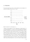
Results and discussion

Steady state

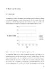
The graph (Figure 5) shows the variation of the overall heat transfer coefficient as a function of the Reynolds referring to the water flowing inside the coil, for constant values of the agitation rate of the bath. These experiments were carried out for steady state conditions and with no insulation of the bath. The bulk temperature of the water in the bath was 33.5ºC.
Figure 5: Steady state U with the bath temperature approximately 33C
The experimental points seen in Figure 5 represent the values of an average of six experiments performed under the same conditions. As seen on the graph (Figure 5) the effect of the Reynolds number is clear . For an agitation rate of 618 rpm and with the change of Reynolds number, Re, from 1993 to 3855 the overall heat transfer coefficient, U, changes from 636 W•m-2•K-1 to 730 W•m-2•K-1. For 980 rpm and Reynolds numbers from 1993 to 3855 the U changes from 687 W•m-2•K-1 to 787 W•m-2•K-1. For an agitation rate of 1342 rpm and for Re being in the range of 1993 to 3855, the overall heat transfer coefficient is in the range of 618 W•m-2•K-1 and 775 W•m-2•K-1. For an agitation rate of 1703 rpm and with the Reynolds number increasing from 1993 to 3855, the global heat transfer coefficient changes from 666 W•m-2•K-1 to 816 W•m-2•K-1. The higher Reynolds number results in higher overall heat transfer coefficient. This is expected because of the velocity of the water inside the coil increases , the convective heat transfer resistance decreases, the internal heat transfer coefficient rises , and consequently so does the overall heat transfer coefficient.
The effect of the agitation rate is not as clear. For a Reynolds number of 1993 and with the change of agitation from 618 rpm to 1703 rpm the overall heat transfer coefficient changes form 636 W•m-2•K-1 to 666 W•m-2•K-1. For a Reynolds number of 2628 and with the agitation changing from 618 rpm to 1703 rpm, the global heat transfer coefficient changes from 661 W•m-2•K-1 to 725 W•m-2•K-1. For the Reynolds number of 3245 with the change of the agitation from 618 rpm to 1703, rpm the overall heat transfer coefficient changes from 688 W•m-2•K-1 to 757 W•m-2•K-1. For the Reynolds number of 3855 and with the change of agitation from 618 to 1703 the overall heat transfer changes from 731 W•m-2•K-1 to 816 W•m-2•K-1. It can be observed , that the heat transfer coefficient with the highest agitation rate of 1703 is higher than with the heat transfer coefficient with the lowest agitation rate of 618 rpm. With other agitation rates there are some anomalies seen, but the differences are very small. The biggest percentage error seen on the graph (Figure 5) is with the Reynolds number of 1993 and between agitation rates of 980 rpm and 1343 rpm, the percentage of the error is 11%. It is expected that higher agitation rates would lead to higher global heat transfer coefficients, because the outside heat transfer coefficient should be higher. However during the present experiments this behavior was not always observed, possibly because the experimental set up used is not a standard one.
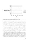
The following graph (Figure 6) shows the results obtained for the overall heat transfer coefficient under steady state conditions and, when the bath was insulated, the temperature of the water in the bath was maintained at 44oC.
Figure 6: Steady state U with the bath temperature approximately 44C
The points seen on the graph (Figure 6) represent the value of an average of three experiments carried out under similar conditions. When analyzing at the graph (Figure 6), the effect of the Reynolds number is evident. For the agitation rate of 618 rpm and for a range of Reynolds number between 1993 and 3855, the overall heat transfer coefficient changes from 551 W•m-2•K-1 to 666 W•m-2•K-1. For the agitation rate of 980 rpm and with the change of Reynolds number from 1993 to 3855 the global heat transfer coefficient changes from 594 W•m-2•K-1 to 715 W•m-2•K-1. For the agitation rate of 1342 and with Re changing from 1993 to 3855, the overall heat transfer coefficient changes from 626 W•m-2•K-1 to 782 W•m-2•K-1. For the agitation rate of 1703 rpm and the Reynolds number changing from 1993 to 3855, the global heat transfer coefficient changes from 594 W•m-2•K-1 to 804 W•m-2•K-1. With the rise of Reynolds number, the global heat transfer coefficient increases as well.
The effect of the agitation is not as clear, but a trend can be seen. With the Reynolds number of 1993 and with the change in agitation rate from 618 rpm to 1703 rpm the overall heat transfer coefficient changes from 551 W•m-2•K-1 to 594 W•m-2•K-1. With the constant Reynolds number of 2628 but with the change of agitation rate from 618 rpm to 1703 rpm the global heat transfer coefficient changes from 607 W•m-2•K-1 to 689 W•m-2•K-1. With the Reynolds number of 3245 and with the change of agitation rate from 618 rpm to 1703 rpm the global U varies from 635 W•m-2•K-1 to 731 W•m-2•K-1. With the highest Reynolds number of 3855 and with the change of agitation rate from 618 rpm to 1703 rpm the overall heat transfer coefficient changes from 666 W•m-2•K-1 to 804 W•m-2•K-1. The highest agitation rate always results a higher global heat transfer coefficient than the lowest agitation rate. The biggest percentage error noticed on the graph Figure 6 can be seen with the Reynolds number of 1993 between the agitations of 1342 rpm and 1703 rpm which is 5, 3%.
When comparing the two charts, Figures 5 and 6, it is expected that the value of the overall heat transfer coefficient should be similar, since the only difference between the experiments was an increase of ten degree in bath temperature.
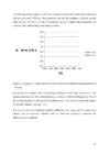
The following graph (Figure 7) shows the comparison between the results of the two experiments in steady state with the same agitation of 618 rpm. One using the insulation, which allowed to use a higher temperature of the bath and one without.
Figure 7: Comparison of steady coefficient of different state heat transfer bath temperatures at 618 rpm.
The difference between the results of the experiments was not very large. With the Reynolds number of 1993 the percentage difference was 15%, with the Reynolds number of 2628 the difference was 9%, with the constant Reynolds number of 3245 the difference was 8% and with the Reynolds number of 3855 the difference was 10%.
The following graph (Figure 8) shows the comparison between the steady state experiments with the agitation of 1703 rpm. One experiment was with the insulation of the bath and the other was not. The result of using the insulation was that a higher bath temperature was achieved, while still reaching steady state conditions.
Figure 8: Comparison of steady state heat transfer coefficient of different bath temperatures at 1703 rpm.
For the Reynolds number 1993 the percentage difference of the value of the overall heat transfer coefficient was 12%, with the Reynolds number of 2628 the difference was 5%, for the constant Reynolds number of 3245 the difference was 2, 4% and for the Reynolds number of 3855 the difference was only 1, 5%.
It is noticed, that the overall heat transfer coefficients were bigger with the experiments without using the insulation, therefore with the lower bath temperature. However, the difference is not significant.

Unsteady state

The following graph (Figure 9) shows the result overall heat transfer coefficient of the unsteady state calculated assuming there was no heat loss.
Figure 9: Unsteady state U considering no heat loss
The points on the graph represent a result from a single experiment in unique conditions. The conditions that varied between the experiments were flow rate and agitation. When looking at the effect of the Reynolds number, a clear trend is seen. With the constant agitation rate of 618 rpm but with the Reynolds number rising from 1993 to 3855, the global heat transfer coefficient rises from 368 W•m-2•K-1 to 521 W•m-2•K-1. With the constant agitation rate of 980 rpm and with the change of Reynolds number from 1993 to 3855, the overall heat transfer coefficient changes from 390 W•m-2•K-1 to 554 W•m-2•K-1. With the constant agitation rate of 1342 but with the Reynolds number rising from 1993 to 3855 the global heat transfer coefficient rises from 435 W•m-2•K-1 to 545 W•m-2•K-1. With the agitation rate of 1703 and with the change of Reynolds number from 1993 to 3855 the global heat transfer coefficient changes from 447 W•m-2•K-1 to 684 W•m-2•K-1. Bigger Reynolds number results in bigger global heat transfer coefficient values.
The effect of the agitation is well seen also. With the constant Reynolds number of 1993 but with the change of agitation rate from 618 rpm to 1703 rpm, the overall heat transfer coefficient changes from 389 W•m-2•K-1 to 448 W•m-2•K-1. With the Reynolds number of 2628 and with the rise of the agitation rate from 618 rpm to 1703 rpm, the global heat transfer coefficient rises from 457 W•m-2•K-1 to 526 W•m-2•K-1. With the Reynolds number constant at 3245 and with the change of agitation rate 618 rpm to 1703 rpm, the overall heat transfer coefficient changes from 500 W•m-2•K-1 to 595 W•m-2•K-1. With the Reynolds number of 3855 and the agitation rate changing from 618 rpm to 1703 rpm, the overall heat transfer coefficient changes from 521 W•m-2•K-1 to 684 W•m-2•K-1. As seen, when comparing the highest and the lowest agitation rates, the trend is evident.
On the following graph (Figure 10) it is shown that in reality there was some heat loss through the bath walls, therefore another way to calculate the global heat transfer coefficient was used.
Figure 10: Bath heat loss
The points on the graph (Figure 10) represent the heat lost in Watts . Two experiments were carried out, one with the agitation of 618 rpm, the other with the agitation of 1342 rpm. As shown, the effect of the agitation to heat loss is not noticed.
The heat loss rate was much higher in the beginning of the experiment, with zero time the heat loss rate was around 214 W. 10 000 seconds later the heat loss rate was less than half , and it was around 75 W. It continued declining but not with such fast rate. After 30 000 seconds the heat loss rate was approximately 35 W. When comparing different agitation rates the heat loss difference is not evident. Another approach to calculate the unsteady state heat transfer was taken and the results from calculations considering no heat loss are acknowledged but dismissed from further comparisons .
On the following graph (Figure 11) are the results of the unsteady state heat transfer calculated by the way when considering heat loss.
Figure 11: Unsteady state U considering heat loss
When investigating Figure 11 the effect of the Reynolds number, Re, to the overall heat transfer coefficient is clear. With the constant agitation rate of 618 rpm but with the increase of the Reynolds number from 1993 to 3855, the overall heat transfer coefficient (U) increases from 477 W•m-2•K-1 to 603 W•m-2•K-1. With 980 rpm and with the change of Re from 1993 to 3855, the U changes from 528 W•m-2•K-1 to 719 W•m-2•K-1. With the constant agitation rate of 1342 rpm and the rise of Re from 1993 to 3855, the global heat transfer coefficient rises from 513 W•m-2•K-1 to 779 W•m-2•K-1. With the highest agitation rate of 1703 and with the change of Reynolds number from 1993 to 3855, the overall heat transfer coefficient changes from 628 W•m-2•K-1 to 839 W•m-2•K-1. The higher velocity of the liquid inside the coil results in higher Reynolds number. Higher Reynolds number results in higher inside coil convective heat transfer coefficient, which causes the overall heat transfer coefficient to rise as well.
The effect of the agitation on Figure 11 is clearest of all the results from the experiments carried out during this particular work. With the constant Reynolds number of 1993, but with the agitation rate changing from 618 rpm to 1703 rpm, the overall heat transfer coefficient changes from 477 W•m-2•K-1 to 628 W•m-2•K-1. With the Re of 2628 and with the increase of the agitation rate from 618 rpm to 1703 rpm, the U increases from 578 W•m-2•K-1 to 731 W•m-2•K-1. For the constant Reynolds number of 3245 and for the change in agitation rate from 618 rpm to 1703 rpm, the global heat transfer coefficient changes from 619 W•m-2•K-1 to 820 W•m-2•K-1. With the constant Reynolds number of 3855 and with the agitation rate rising from 618 rpm to 1703 rpm, the overall heat transfer coefficient rises from 603 W•m-2•K-1 to 839 W•m-2•K-1. It is expected, that with higher agitation rates the overall heat transfer coefficient is higher as well. Since higher agitation rates reduce the convective heat transfer resistance outside the coil, increasing the convective heat transfer coefficient. This influences the overall heat transfer coefficient. As seen on Figure 11, in this case the expected can be observed.
It is expected, that the results from steady state experiments and unsteady state experiments are similar. In the following graph (Figure 12) results for the experiments of steady state with insulation and unsteady state considering heat loss are compared. For clarity only the lowest agitation rate of 618 rpm and the highest agitation rate of 1793 are compared.
Figure 12: Comparison of steady state and unsteady state heat transfer coefficient at agitations of 618 rpm and 1703 rpm.
When the results of steady state and unsteady state experiments are compared with the constant agitation rate of 618 rpm, the percentage difference between them at the Reynolds number of 1993 is 15%. When the Re is 2628, the percentage difference is 5%, With the Reynolds number of 3245 and with the same agitation rate of 618 rpm, the percentage difference is 2, 5%. With the Reynolds number of 3855 at the agitation rate of 618 rpm, the percentage difference is 10%. When investigating the highest agitation rate of 1703 rpm, the results are similar. With Reynolds number of 1993, the percentage difference is 5%.At Reynolds number of 2627, the percentage difference is 6%. With the Re of 3245, the percentage difference is 11% and with Re of 3855, the difference in percentage is 4, 4%. The differences between the results of two experiments are not very large; therefore it is believed that the results are satisfactory.

Theoretical

Theoretical result for the overall heat transfer coefficients were calculated with empirical equations. One set of equations were taken from a book by Richardson and Coulson.
The following graph (Figure 13) shows the theoretical overall heat transfer coefficient values calculated with equation by Richardson and Coulson.
Figure 13: Theoretical heat transfer coefficient according to Richardson and Coulson
After investigating the results from Figure 13, another source for the empirical equations to use when calculating the theoretical overall heat transfer coefficients was chosen. The empirical equations by Geankoplis give closer results to the experimental results (which can be seen on Figure 14) than the ones by Richardson and Coulson. Therefore the theoretical results from Richardson and Coulson are acknowledged but dismissed from further comparison.
Figure 14: Theoretical heat transfer coefficient according to Geankoplis.
Theoretical numerical results calculated with data from different authors , differ slightly, but the trend is clearly seen on Figure 13 and Figure 14. The overall heat transfer coefficient is bigger with higher Reynolds number and the effect of the agitation is also very straight forward . Overall heat transfer coefficient is higher with faster agitation rates.
The results, of the overall heat transfer coefficients for the coil should be similar with all the experiments. When investigating the change of overall heat transfer coefficients between different experiments a similar trend can be found with all the experiments. For the steady state with the bath at 44oC (Figure 6), the heat transfer coefficient changes from 551 W•m-2•K-1 to 804 W•m-2•K-1. For unsteady state calculated with equations, that do consider heat loss (Figure 11), the overall heat transfer coefficient differs from 477 W•m-2•K-1 to 839 W•m-2•K-1 According to (Geankoplis, 1993) the overall heat transfer coefficients (Figure 14) varies from 627 W•m-2•K-1 to 1180 W•m-2•K-1. The theoretical values from Table 1 suggests that the number of overall heat transfer coefficient while cooling the water inside the bath should be between 250 W•m-2•K-1 and 800 W•m-2•K-1.
A common trend can be seen in all the graphs, the heat transfer coefficient grows with higher agitation rates and with higher Reynolds number. The experimental results do not show the effect of the agitation as clearly as expected, but the effect of the Reynolds number is certain. When comparing the numerical values of experimental and theoretical overall heat transfer coefficient results, it is seen, the difference is rather large, the theoretical results overpredicts the value of overall heat transfer coefficient by 31% to 41%. The biggest difference in percentage terms between the lowest U of experimental results (Figure 11) and theoretical results (Figure 14) is 31%. The biggest difference between the highest experimental U (Figure 11) and the highest experimental U (Figure 14) is 41%.
It may be caused by multiple things, but the most obvious seems to be, that the difference comes from the outside convection. To use the equation to calculate theoretical outside convection, many modifications were used. The equation was meant to be used with paddle agitators and in a cylindrical tank with no baffles, in this case, the tank was rectangular. Instead of a diameter, an equivalent diameter was used. The agitator that was used to carry through this particular experiment was not considered as „standard“ as you can see on the Figure 4Error: Reference source not found, it is more close to a turbine than a paddle. It is believed that the effect of the agitator speed in the experiment does not match the effect expected while engaging empirical equations from the literature. Due to the turbine agitators blades were small; the effect of the agitation is thought to be a lot less that the equivalent paddle agitator.
The experimental results fit the values given in Table 1 by Fletcher. The values of overall heat transfer coefficients in case of internal coil and cooling of the bath as can be seen in Table 1 are between 250 W•m-2•K-1and 800 W•m-2•K-1, which can also be seen in the experimental results. U grows bigger than the number of 800 W•m-2•K-1 only on rare occasions, most of the results stay in the boundaries given by Fletcher.

Conclusions and suggestions for future work

From the experimental work carried out, conclusions can be made:

• The heat transfer coefficient is mostly formed by convective heat transfers, rather than conduction. This means, that when exchanging heat between two fluids through a low heat resistance coil, the key things to improve overall heat transfer coefficient are to increase the Reynolds number inside the coil and the agitation in the bulk fluid.
  
• The Reynolds number inside the coil affects the convection heat transfer coefficient proportionally. In fact in many cases the effect of the Reynolds number on the overall heat transfer coefficient was found to be linear.
  
• In this experiment, the effect of the agitator was not drawn out very clearly. Although , it was seen that when the highest (1703 rpm) and the lowest (618 rpm) agitation rates were applied, the overall heat transfer coefficient was always higher with the highest agitation rate of 1703 rpm than the one with the lowest agitation rate of 618 rpm. Therefore it is believed that the agitation inside the bath increases the overall heat transfer coefficient, but it is not very sensitive to small changes in agitation.
  

For future work, it is suggested to use a „standard“ agitator blade and as well a „standard“ bath, for which there are more equations to be found in the literature therefore a more reliable comparison with the theoretical results can be made. Another detail, which could make the experiment more consistent, is fixing the coil, also fixing the space between the coil’s spirals. It might be interesting to understand, by which correlation the Reynolds number inside the coil changes the overall heat transfer coefficient.

Bibliography

Coulson, J. M. & Richardson, J. F., 2004. Coulson and Richardson's Chemical Engineering Volume 1 - Fluid Flow, Heat Transfer and Mass Transfer.
Fletcher, P., 1987. Heat transfer coefficients for stirred batch reactor design.
Geankoplis, C. J., 1993. Transport Processes and Unit Operations, Third Edition.
Hewitt, G. F., Shires, G. L. & Bott, T., 1994. Process Heat Transfer, chapter 31.
Jeschke, D., 1925. Wärmeübergang und Druckverlust in Rohrschlangen.
http://www.thermopedia.com/content/1176/

APPENDICES

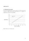
A.1 Calibration of the rotameter

The rotameter was calibrated using a timer and a scale . The value of the rotameter was set to constant and the amount of water went through the system was scaled. The points on the graph represent an average of three measurements.
Figure 15: Calibration curve for the rotameter

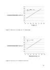
A .2Calibration of Thermocouple and Electronic thermometer

The thermocouples and the electronic thermometer were calibrated with pre-calibrated mercury thermometer. The temperature of the water inside the bath was changed and all the thermometers were placed into the water at same temperature, while changing temperature of the water, calibration curves for the thermocouple and electronic thermometer were formed.
Figure 16: Calibration curve for the outlet (T1) thermocouple.
Figure 17: Calibration curve for the inlet (T2) thermocouple.

Figure 18: Calibration curve for electronic thermometer

A.3 Calculation example

The following calculation example is shown, how heat transfer coefficient was calculated for steady state heat transfer with the flow rate of 0,008556 kg/s and with the agitator in position 8, or at 1703,41 rpm.
The equations (1) and (2) were used.
From equation (2), the amount of heat exchanged is calculated:
This is inserted to equation (1)
The logarithmic mean temperature was calculated by equation:
(0)
Calculations for unsteady state considering there is no heat loss are following.
Using the equation (15) a calculation example is shown for unsteady state with flow rate 0,00574 kg/s and with the agitation at 617,83 rpm.
To calculate the heat transfer coefficient considering the heat loss, a little different approach was taken. Using the equation following, the amount of heat gained in the coil was calculated.
Then, the calculated value of Q was replaced into equation
and with the series of results on the same agitation rate and flow rate, in this case flow rate 0,0057 kg/s and agitation 617,83 rpm a linear graph was conducted., where y equals to Q and x equals to A•∆Tlm which makes k equal to U.
In the case examined here the variables of linear function conducted.
y
x
1224,004
1,894311
1082,748
1,798533
939,0853
2,112095
850,5479
1,810088
752,403
1,598259
649,659
1,576971
606,5281
1,164128
539,5923
1,150495
482,2187
1,164068
432,0168
0,959698
384,1552
0,855494
336,3992
0,783912
298,161
0,754559
278,9918
0,598414
250,3591
0,556669
226,4072
0,521141
200,1129
0,565006
180,9888
0,531864
161,8325
0,544722
From these variables a linear function was formed and on the graph the slope is equal to the overall heat transfer coefficient, U.
To calculate the theoretical overall heat transfer coefficient an equation (18) was used, which represents the connection between resistance and heat transfer coefficient. An example is shown for reading at the flow rate of 0,00866 kg/s and at the agitation rate at 1703,41.
The convection inside coil was calculated with the equation (20), an equation (21) was fitted because equation (20) is for straight pipes and equation (21) correlates it to coil.
Calculation for the critical Reynolds number is based on the equation (19) the following:
The Nusselt number was calculated using the following formula (28). When using the equation (20) it is considered, that inside the coil there was a laminar flow.
(0)
The correlation between a straight pipe and a coil.
To calculate the convection outside coil was a bit more difficult, because of the large amount of variables. Nevertheless an equation (22) was found in a book from Richardson and Coulson which was exactly about convection outside coil. It should be noted, that this formula is meant to be used with square tanks, the one in experimental setup was rectangular.
Another equation (23) to calculate the theoretical outside coil convective heat transfer coefficient was found by Geankoplis.