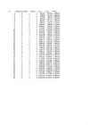
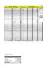
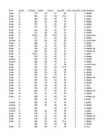
Standard Error 1160,052615 Observations 35 ANOVA df SS MS F Significance F Regression 1 397496237,381 397496237,4 295,37766127 4,969708E-018 Residual 33 44408828,2678 1345722,069 Total 34 441905065,649 Coefficients Standard Error t Stat P-value Lower 95% Upper 95% Lower 95,0%Upper 95,0% Intercept 429,600229 245,692413075 1,748528673 0,0896708332 -70,264741368 929,4651993 -70,26474 929,4651993 X Variable 1 0,73444368 0,0427336191 17,18655467 4,96971E-018 0,6475014786 0,821385881 0,647501 0,821385881 90% Usaldusvahemik Usaldusvahemik: Alumine piir Ülemine piir Tulu: 2 112,47 ; 4 663,98 Kulu: 1909,95705 ; 3885,80581 Palk: 3406,73204 ; 8467,7251
signaali erinevus detsibellides. Minimaalne signaali tase oleneb analüsaatori omamürast, maksimaalne tase aga analüsaatori lineaarsusest ja moonutuste tekkimisest suure sisendsignaali korral. d) Kuidas paiknevad spektris 2. ja 3. järku moonutussaadused? f1 ja f2 on lähestikku paiknevad testtoonid. Näiteks 200 MHz ja 201 MHz. 2. järk: 2*f1; 2*f2; f1±f2 3. järk: 3*f1; 3*f2; 2*f1±f2; f1±2*f2 e) Mida iseloomustab parameeter third order intercept point TOI? TOI on siinussignaali suurus, mille juures tekkiv 3. järku moonutus on sama suur kui sisendsignaal. Töö käik 2 1. Jälgisime analüsaatori abil antud sagedusega siinussignaali spektrit. Selleks seadsime generaatori HP33120A väljundsignaali kujuks siinuse, mille amplituud oli 50 mV ja sagedus 90 kHz-i. Ühendasime signaali analüsaatori sisendile ja valisime analüsaatori jaoks parameetrid, mis sobiksid
points(h~d_k,data=subset(PD.KU),lwd=1) with(subset(PD., pl=="KU"),rug(d_k)) 1. Sirge h=a+b*d M1 <- lm(h~d_k, data=PD.KU) summary(M1) D<-0:40 M1.pred <- predict(M1,newdata=data.frame(d_k=D)) lines(D,M1.pred, col="red") coefficients(M1)[1] coefficients(M1)[2] # dobavit' p-value v tablicu v vide * summary(M1)$adj.r.squared summary(M1)$sigma # sqrt(sum(M1$residuals^2)/(length(M1$residuals)-2)) AIC(M1) > coefficients(M1)[1] (Intercept) 7.758512 > coefficients(M1)[2] # dobavit' p-value v tablicu v vide * d_k 0.5027412 > summary(M1)$adj.r.squared [1] 0.7619479 > summary(M1)$sigma # sqrt(sum(M1$residuals^2)/(length(M1$residuals)-2)) [1] 1.823029 > AIC(M1) [1] 177.6237 2. Ruutparabool h=a+b*d+c*d^2 M2 <- lm(h~d_k + I(d_k^2), data=PD.KU) summary(M2) M2.pred <- predict(M2,newdata=data.frame(d_k=D)) lines(D,M2.pred, col="blue") coefficients(M2)[1] coefficients(M2)[2] coefficients(M2)[3] summary(M2)$adj.r
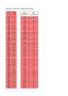
11,5 10 10 Standard Error 2,056276 9,3 5 2 Observations 10 6 4 6 12,2 10 18 ANOVA df SS MS Regression 1 233,84283 233,84283 intercept on 0 Residual 8 33,826167 4,2282709 Total 9 267,669 CoefficientsStandard Error t Stat Intercept 0,1005168 1,267315 0,0793148 Koopia-masinate arv 1,4192076 0,1908382 7,4367063
0,050087 Observations 20 ANOVA df SS MS F Significance F Regression 1 7,797748 7,797748 3108,303 1,3E021 Residual 18 0,045156 0,002509 Total 19 7,842905 Coefficients Standard Error t Stat Pvalue Lower 95%Upper 95% Lower 95,0% Upper 95,0% Intercept 0,02403 0,023267 1,03285 0,315351 0,07291 0,024851 0,07291 0,024851 X Variable 10,02166 0,000388 55,7522 1,3E021 0,02247 0,02084 0,02247 0,02084 SUMMARY OUTPUT Regression Statistics Multiple R 0,997434 R Square 0,994874 Adjusted R Square 0,994589 Standard Error 0,040604 Observations 20 ANOVA df SS MS F Significance F Regression 1 5,760008 5,760008 3493,664 4,5E022 Residual 18 0,029677 0,001649
Standard Error 5,684885887 Observations 145 ANOVA df SS MS F Regression 9 18483,362517209 2053,706946357 63,5469877603 Residual 135 4362,9202190334 32,3179275484 Total 144 22846,282736242 Coefficients Standard Error t Stat P-value Intercept 45,2325050445 4,5122271955 10,0244298625 5,0841941E-018 X2 54,0929506547 23,6488063569 2,2873438024 0,023730954 X3 -5,1644389493 1,0898051827 -4,7388643688 5,3785349E-006 X4 -4,5777656267 0,5803114144 -7,8884638711 9,2683831E-013 X5 0,0246916715 0,0390769079 0,6318737289 0,5285379712
Observations 37 ANOVA df SS MS F Regression 4 5452896,128908 1363224 2,068745 Residual 32 21086782,96908 658962 Total 36 26539679,09799 Coefficients Standard Error t Stat P-value Intercept 316,8447162072 515,1894957149 0,615006 0,5429 X1 0,3616205503 0,2486257171 1,454478 0,155553 X2 325,0756415193 419,6871545439 0,774567 0,444282 X3 -1,1237269925 1,0313144227 -1,089607 0,284024 X4 0,0005921042 0,0003028169 1,955321 0,059326 RESIDUAL OUTPUT
856476112 Standard Error 197.413872 Observations 18 ANOVA df SS MS Regression 1 3992595.82144818 3992595.821 Residual 16 623555.789662928 38972.23685 Total 17 4616151.61111111 Coefficients Standard Error t Stat Intercept 3076.114111 99.2070711068 31.00700461 Väärtus jooksevhindades, miljoni-0.097903113 0.0096726727 -10.12161951 F Significance F 102.447181 2.3209959E-008 P-value Lower 95% Upper 95% Lower 95,0% Upper 95,0% 1.0199E-015 2865.80451528 3286.423707 2865.804515 3286.4237068 2.3210E-008 -0.1184082627 -0.07739796 -0.118408263 -0.077397963 punktide arv intervalli alapiir intervalli ülapiir Õpilaste arv
ANOVA df SS MS F Significance F Regression 1 1347945730.06 1347945730.06 340.60658825 1.044501E-010 Residual 14 55404800.9395 3957485.78139 Total 15 1403350531 Coefficients Standard Error t Stat P-value Lower 95% Intercept 0 Err:512 Err:512 Err:512 Err:512 Töötajate arv (tuh) 235 13 18 0 208 SUMMARY OUTPUT Regression Statistics Multiple R 0.9848934499 R Square 0.9700151077 Adjusted R Square 0.8907855006 Standard Error 1799.1304432266 Observations 15 ANOVA
ESS Regression 1 981245 RSS Residual 3 15875 TSS Total 4 997120 Coefficients Standard Error Intercept -488,5 246,1495141846 Perede arv (X) 0,443 0,0325320355 Sa1 RESIDUAL OUTPUT Observation Predicted Autode arv Y Residuals 1 2612,5 -92,5 2 2834 26 3 3055,5 -35,5 4 2169,5 60,5 5 3498,5 41,5 utada
ANOVA Significance df SS MS F F Regression 1 107,3533 107,3533 60,92444 5,39E-09 Residual 33 58,14841 1,762073 Total 34 165,5017 Coefficients Standard Error t Stat P-value Lower 95% Intercept 5,502895 0,707134 7,781965 5,75E-09 4,064219 d 0,452119 0,057924 7,805411 5,39E-09 0,334272 Regr. Võrrand h=5,5029+0,4521*d Jah. Regressioonivõrrand on sama mis graafikul. Regressioonivõrrand on usaldatav. 22. 1 Jääkstandardhälve ja kõrguse standardhälve Jääkstandardhälve iseloomustab funktsioontunnuse keskmist erinevust regressioonijoonest Tabel 8 Võrrandi jääkstandardhälve ja kõrguse standardhälve
934,052 Residual 155 1 6,02614256 1286,47 Total 160 2 CoefficientStandar Upper Lower Upper s d Error t Stat P-value Lower 95% 95% 95,0% 95,0% 143,662 4,39506340 915,195 915,195 Intercept 631,40632 6 4 2,04558E-05 347,617 6 347,617 6 - 0,07145 4,35708932 aasta -0,311329 3 9 2,3883E-05 -0,45248 -0,17018 -0,45248 -0,17018 0,52676 0,15034420 0,88068852 1,11976 1,11976
Observations 50 vaatluspunktide arv 1,98%. ANOVA df SS MS F Significance F Regression 1 1,15015E+017 1,2E+017 1,990401 0,1647474991 Residual 48 2,77367E+018 5,8E+016 Total 49 2,88868E+018 Coefficients Standard Error t Stat P-value Lower 95% Upper 95% Intercept 94575011,592 37913746,956 2,494478 0,01611 18344315,5246 1,7E+008 X1 8,3099697405 5,8901885958 1,410816 0,164747 -3,5330479689 20,15299 Y ja X1 hajuvusdiagrmm 40000000 30000000 X1 Paarisregressioonivõrra
what it is that your doing. So he studid all these books therefore he knew Unix system and C programming like the back of his hand. James committed a series of intrusions into various systems, like BellSouth and the Miami- Dade school system. What brought him to the attention of federal authorities, however, was his intrusion into the computers of the Defense Threat Reduction Agency. As hacking into these systems he was allowed to intercept over three thousand messages passing to and from DTRA employees. On June 29 and 30, 1999, this young hacker made a mess of NASA He gained access by breaking the password of a server belonging to the government agency located in Alabama. He was able to freely roam the network, and stole several files, including the source code of the International Space Station. According to NASA, the value of the documents stolen by James was estimated at around $1.7 million
tabeli korral menüüst valida Tools, Data Analysis, Regression. Sellise valiku tulemusena avaneb sisestusaken, milles saab määrata funktsiooni y väärtuste ploki (Input Y- Range), argumendi x väärtuste ploki (Input X Range), usaldusnivoo (Confidence Level) ja selle koha, kuhu tulemused väljastatakse (Output options). Regressioonanalüüsi protseduuri rakendamise tulemusena tekib kolm tabelit, millest viimases on antud vabaliige (Intercept) koos oma standardmääramatusega (Standard Error) ja sirge tõus (X Variable) koos oma standardmääramatusega. Graafik tuleb teha eraldi – eelneva protseduuriga graafikut ei joonestata.
Olgu palk sõltumatu tunnus – x ja kulu spordile sõltuv tunnus -y. Koostada hajuvusdiagramm. Koostada lineaarse regressiooni võrrand. Leida kogu-, jääk- ja regressioonhajuvus. Kui suure osa koguhajuvusest moodustab regressioonhajuvus? Kas see on oluline? Hajuvusdiagrammi sain OpenOffice XY(scatter) joonise abil, kus x-teljel on palk ning y-teljel kulutused spordile. Lineaarse regressiooni leidmiseks on vaja leida a ja b, vastavalt Kuid mis on leitavad ka OpenOffice funktsioonide INTERCEPT ja SLOPE abil. Vastavad tulemused tulid: a = -60.8243633 b = 0.139701932 ja seega võrrand on ŷ = a + bx ehk ŷ = -60.8243633 + 0.139701932x Kuna OpenOffice, kuigi suutlik andmeanalüüsi juures, jõudsin lahendusteni, milles ma ei olnud kindel, seega viimane uurimus sai tehtud kursakaaslase abil Excelis. Regerssioonihajuvuse osa koguhajuvusest: SSR/SST = 0.875 = 87.5% Võime järeldada, et lineaarne regressioonimudel iseloomustab vaatlusandmeid hästi.
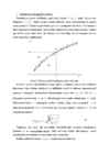
511991 Standard Error 0.721537 Observations 20 ANOVA df SS MS F Significance F Regression 1 10.89841 10.89841 20.9337 0.000235 Residual 18 9.371086 0.520616 Total 19 20.2695 Coefficients Standard Error t Stat P-value Lower 95%Upper 95%Lower 95,0% Upper 95,0% Intercept 3.850082 0.444476 8.662071 7.8E-008 2.916272 4.783891 2.916272 4.783891 X Variable 1 0.284736 0.062233 4.575336 0.000235 0.15399 0.415482 0.15399 0.415482 12 Dkesk 10 f(x) = 1.8883297565x - 4.1934544513 8 R² = 0.5376755398
Regression 1 16,68045478 16,68045 48,71302735 6,45445E-06 Residual 14 4,793920222 0,342423 Total 15 21,474375 Upper Coefficients Standard Error t Stat P-value Lower 95% 95% Intercept 3,902516762 0,531490252 7,342593 3,66132E-06 2,762583548 5,04245 X Variable 1 0,409323758 0,05864681 6,979472 6,45445E-06 0,283538861 0,5351087 27) Kuna P value on väiksem kui 0,05 siis regressioonvõrrand on usaldatav. 28) Saadud võrrandi jääkstandardhälve on 0,59m. Kõrguse standardhälve on1,20m. Jääkstandardhälve e. prognoosiviga iseloomustab funktsioontunnuse erinevust regressioonijoonest.
Observations 30 ANOVA df SS MS F Significance F Regression 1 513,330843841 513,330844 2,599690801 0,1181007 Residual 28 5528,83582283 197,458422 Total 29 6042,16666667 Coefficients Standard Error t Stat P-value Lower 95% Intercept 11,6756701836 27,0953075954 0,43091115 0,669832231 -43,8265507 Gümn_keskmHinne 10,0798045001 6,2516011193 1,61235567 0,118100702 -2,72601971 Korrelatsioonikordaja SEOS tr= 1 0,291 nõrk 1,612
Regression 1 3,2827547444 vabaliige -2,0057989331 Residual 8 0,5024741556 tõus 0,0588035857 Total 9 3,7852289 Coefficients Standard Error vabaliige Intercept -2,005799 1,6744575692 tõus a Läbimüük, tuh. kr 0,0588036 0,0081338557 mudelit otsitakse kujul y= ax + b a) Tootmisvarude sõltuvust läbimüügist kirjeldab mudel Y=0,059X - 2,006,
Residual 290 30,64322 Väga usaldusväärne Total 299 Upper Coefficients t Stat P-value Lower 95% Upper 95% Lower 95,0% 95,0% Intercept 13,35620356 8,842238 9,32E-17 10,38326958 16,32913755 10,38326958 16,32913755 Piimalehmad, keskmine arv 0,002010385 0,225657 0,821627 -0,015524144 0,019544915 -0,015524144 0,019544915 Koresööda kogus looma kohta 0,000243501 2,08012 0,038393 1,3104E-05 0,000473898 1,3104E-05 0,000473898
called My Mother's Hymn Book. He was also significantly influenced by traditional Irish music that he heard performed weekly by Dennis Day on the Jack Benny radio program. Cash enlisted in the United States Air Force basic training at Lackland Air Force Base and technical training at Brooks Air Force Base, both in San Antonio, Texas. Cash was assigned to a U.S. Air Force Security Service unit, assigned as a code intercept operator for Soviet Army transmissions at Landsberg, Germany. Where he created his first band named The Landsberg Barbarians. He was the first radio operator to pick up the news of the death of Joseph Stalin. After he was honorably discharged as a Staff Sergeant on July 3, 1954, he returned to Texas. On August 7, 1954, one month after his discharge, he married his first wife, Vivian Liberto, in San Antonio. In 1954, Cash and Vivian moved to
Telgede muutmiseks Select data-Edit. Nimeta teljed, võta pealkiri ära, eemalda jooned, muuda suurused telgedel, muuda punktid selgemaks. Regressioonisirge lisamiseks Chart Layout Trendline Linear trendline. Andmete lisamiseks graafikult, parem klõps Format trendline ja kaks alumist ticki teha. Tee regressioonanalüüs: Data analysis: regression. Seejärel pane paika võrrand, a+b*otsitav; a ja b saad regressioonitabelist. a=intercept ja b on selle all. Seejärel püstita hüpoteesid: H0: regressioonivõrrand ei ole statistiliselt oluline; H1: regressioonivõrrand on statistiliselt oluline. P väärtus on ANOVA all, significance F. NÄITED: Prognoosige hinge kinni pidamise võimet kehalise võimekuse testi abil, Prognoosige tudengite massi nende pikkuse abil. Kui palju võiks keskmiselt kaaluda 170 cm pikkune tudeng? Prognoosige pikkust jalanumbri alusel. Hiiruut-test: Vt ka PRAKS 7
3 N=11 y = x·y x2 = 64,9779 =0,1933 0,00009085 1 Graafikud: 1.) Arvtutused: 2.) Arvutan empiirilise võrrandi ln p=A+B/T koeffitsiendid A ja B logaritmilise graafiku tõusu abil. A= -3792,16 , kasutades funktsiooni SLOPE B=17,356, kasutades funktsiooni INTERCEPT 3.) Arvutan aine auramissoojus, arvestades , et 4.) Arvutan aine keemistemperatuuri normaalrõhul 5.) Arvutan Troutoni konstandi ehk entroopia muudu 1 mooli aine aurustumisel normaalrõhul Katses ma kasutaasin benseeni orgaanilise ainena. Seega, benseeni keemistemperatuur normaalrõhul on 353,3 K. Arvutan viga: Benseeni Troutoni konstant on tegelikult 89,45 J/K*mol. Arvutan viga: Järeldused.
Regression 1 257.66725 257.66725 Residual 39 272.2308 6.9802769 Total 40 529.89805 Coefficients Standard Error t Stat Intercept 73.944794 0.8677696 85.212474 X Variable 1 0.0001347 2.22E-005 6.0756575 parameetrid a ja b käsitsi a ja b funktsiooniga a 73.944794 a 73.944794 b 0.0001347 b 0.0001347 yi koguvariatsioon 529.89805
xi yi (xi-x)^2 3,1 12,1 0,0036 4,9 23,9 3,4596 4,2 16,8 1,3456 1,9 9,2 1,2996 1,1 7,8 3,7636 keskmin e 3,04 13,96 kokku 9,872 Excel: INTERCEPT Excel: SLOPE Regressioonimudel: y=1,94+3,96x 10.2 leida mudeli parameetrite hinnangute b0 ja b1 usaldusvahemikud r 4,3 5,6 3,7 7,2 3,2 4,9 6,6 5,07142 y0 9 2,19238 s²(y) 1 Hinnangu b0 usaldusvahemik: Hinnangu b1 usaldusvahemik: 10
He has not, however, because Amalia and her henchmen kidnap Fandorin from his hotel room. Amalia leaves her henchmen to kill Fandorin, and they are about to do so when Count Zurov appears out of nowhere and saves Fandorin's life. Zurov admits to Fandorin that jealousy over Amalia led him to follow Fandorin to London. Fandorin assures Zurov that he is no rival for Amalia, and Zurov leaves to either kill her or "take her away somewhere". Meanwhile, Fandorin hurriedly leaves for St. Petersburg to intercept the letter that Amalia has mailed to her Azazel contact there. He succeeds, and sees the letter delivered to Gerald Cunningham, a teacher at the Moscow Astair House. Fandorin reports this to Brilling, and they go together to arrest Cunningham--but Brilling shoots Cunningham dead, and reveals to Fandorin that he is also an agent of Azazel. Fandorin and Brilling struggle, and Brilling is killed. Fandorin travels back to Moscow to continue the investigation
10.1 leida mudeli parameetrite hinnangud b0 ja b1 xi yi (xi-x)^2 4,9 8,8 3,3124 2,2 0,4 0,7744 4,3 4,6 1,4884 1,2 1,3 3,5344 2,8 0,7 0,0784 keskmin e 3,08 3,16 kokku 9,19 Excel: INTERCEPT Excel: SLOPE Regressioonimudel: y=2,03x-3,09 10.2 leida mudeli parameetrite hinnangute b0 ja b1 usaldusvahemikud r 4,3 5,6 3,7 7,2 3,2 4,9 6,6 5,07142 y0 9 2,19238 s²(y) 1 Hinnangu b0 usaldusvahemik: Hinnangu b1 usaldusvahemik: 10
Attenuators The axis of attenuator systems is perpendicular to wave front. As a wave hits the device, energy is gradually drawn into the attenuator. A leading buoy and an anchor are used to permit swinging with the waves and orienting to wave direction A typical technology using the attenuating method is sea snake (Pelamis) technology. Terminators A terminator is a horizontally or with a small angel to water surface oriented device to intercept the waves. It has a leading buoy and an anchor to pivot if wave direction changes. 13 A terminator is a horizontally or with a small angel to water surface oriented device to intercept the waves. It has a leading buoy and an anchor to pivot if wave direction changes. Terminators can harvest a lot of the wave energy. For example: a 300 m device in kW
( )( ) ( ) Excel: SLOPE ( ) Excel: INTERCEPT 9.2 leida mudeli parameetrite hinnangute b0 ja b1 usaldusvahemikud. ( ) ( ) ( ) ( ) ( )
sissetulek väheneb 3,57 võrra) Oluline on R2 ehk kui suure osa kogu ennustatava muutuja variatiivsusest kirjeldab ära prediktor. ANOVA tabelis ennekõike oluline p-väärtus <0,05, mis näitab, kas mudel on statistiliselt oluline. Koefitsentide tabeli põhjal saab ehitada regressioonivõrrandi (Uuring nr 2:) Coefficients Mode Unstandardized Standard Error Standardized t p l H₁ (Intercept) 331.581 1.883 176.120 <.001 AGE_R -1.021 0.044 -0.345 -23.115 <.001 Vanuse regressioonikordaja ehk tõus on -1,02 ehk kui vanus suureneb ühe ühiku võrra, väheneb probleemilahendusoskus 1,02 punkti võrra. Standardiseeritud ühikutes on tõus -0,345 ehk kui vanus suureneb ühe ühiku võrra, väheneb probleemilahendusoskus 0,345 standardhälbe võrra. p<
1,0 5,5 4,4 5,0 0,2 4,4 3,0 1,2 0,0 2,0 3,5 1,0 Keskmine 3,0 2,1 Kokku 10,0 Excel: INTERCEPT Excel: SLOPE Regressioonimudel: y = 6,3 1,4x 11.2. Leida mudeli parameetrite hinnangute b0 ja b1 usaldusvahemikud r 3.0 6,3 3,9 2,0 2,7 4,6 3,3 yo 3,69 S2(y) 2,02 Hinnangu b0 usaldusvahemik: Hinnangu b1 usaldusvahemik: 11.3
xi yi (xi-x)^2 1,2 1,3 3,534 4,3 4,6 1,488 4,9 8,8 3,312 2,8 0,7 0,078 2,2 0,4 0,774 Keskmi ne 3,08 3,16 Kokku 9,188 Excel: INTERCEPT Excel: SLOPE Regressioonimudel: y = -3,09+2,03x 11.2 leida mudeli parameetrite hinnangute b0 ja b1 usaldusvahemikud = 2,08 Excel: VAR r 7,1 3,6 5,6 6,4 4,8 3,2 4,3 y0 5 s²(y) 2,07667
Drake out to destroy the Spanish Armada. England's increasing population created new markets and brought about the exploitation of new sources of raw materials, among them those of the New World. The commercial ventures of the Virginia Company in North America and of the East India Company in the Orient were aspects of this expansion. Riches also came from ventures like those of the pirate-patriot Sir Francis Drake, whom Elizabeth commissioned to intercept Spanish treasure ships on the high seas and relieve them of the heavy burden of gold they had stolen from the Indians of South America. 11. The development of poetry during the Elizabethan time. The queen loved music and dancing and her court entertainments were notable. Elizabeth was not only a master politician but also a poet of no mean ability. Most famous of the courtier poets were the Earl of Essex, Sir Walter Raleigh, and Sir Philip Sidney. Edmund
ANOVA df SS MS F Significance F Regression 4 14233112 3558278 73,7379 1,69E-032 Residual 130 6273248 48255,75 Total 134 20506360 Coefficients Standard Error t Stat P-value Lower 95% Intercept -1916,899217 238,9411 -8,022475 5,30E-013 -2389,616 x1 30,890119453 5,350517 5,773296 5,42E-008 20,30476 x2 6,6876682557 2,381831 2,807785 0,005758 1,975501 x3 11,040861678 2,719814 4,059418 8,44E-005 5,660035 x4 1548,4425989 121,5685 12,7372 1,27E-024 1307,934 RESIDUAL OUTPUT
(võttes vastavates testides jm arvutustes olulisuse nivooks a = 0.05): 11.1 leida mudeli parameetrite hinnangud b0 ja b1 Keskmine Xi 5,1 2,8 1,1 2,2 4 3,04 yi 15,3 6,9 7,2 6,1 9,8 9,06 Excel: INTERCEPT Excel: SLOPE Regressioonimudel: 11.2 leida mudeli parameetrite hinnangute b0 ja b1 usaldusvahemikud r y0 3,6 2,6 1,3 0,2 1,9 0,7 4,2 3,6 2,07 2,19 Hinnangu b0 usaldusvahemik: Hinnangu b1 usaldusvahemik: 11
10. Protseduur Regression SUMMARY OUTPUT Regression Statistics Multiple R 0.940941045 R Square 0.885370049 Adjusted R Square 0.881276123 Standard Error 1401.579976 Observations 30 ANOVA df SS Regression 1 424835227.446 Residual 28 55003940.021 Total 29 479839167.467 Coefficients Standard Error Intercept 5767.471447 740.827303296 X Variable 1 1.341186029 0.0912003793 11. Kasutatud materjalide loetelu 1 Kodutöö E4 juhend statistika_kodutoo_juhend_2017_kaug.pdf 2 korrelatsioonikordajad.xls 3 punkthinnangud.xlsx 4 regressioonanalyys2.xls 5 Kriitiliste punktide jaotus tabelhttp://kontromat.ru/?page_id=4200 6 AnalysisToolPak 2016 https://www.youtube
3,00 3,70 13,10 48,47 13,69 171,61 0,72 2,04 1,47 0,52 4,16 4,00 2,20 6,80 14,96 4,84 46,24 -0,78 -4,26 3,32 0,61 18,15 5,00 1,10 7,20 7,92 1,21 51,84 -1,88 -3,86 7,26 3,53 14,90 14,90 55,30 194,70 9,19 109,77 keskm. 2,98 11,06 Excel: INTERCEPT Excel: SLOPE Regressioonimudel: y=1,36+3,25x 11.2 leida mudeli parameetrite hinnangute b0 ja b1 usaldusvahemikud r yr yr-r (yr-r)2 1,00 4,20 -0,76 0,57 2,00 5,50 0,54 0,29 3,00 3,40 -1,56 2,42 4,00 7,10 2,14 4,59 5,00 3,20 -1,76 3,09 6,00 4,90 -0,06 0,00 7,00 6,40 1,44 2,08 34,70 13,06
circuit. It was addressed to the Japanese embassy, and Bainbridge reached up and snared it as it flashed overhead. The message was short, and its radiotelegraph transmission took only nine minutes. Bainbridge had it all by 1:37. The station's personnel punched the intercepted message on a teletype tape, dialed a number on the teletypewriter exchange, and when the connection had been made, fed the tape into a mechanical transmitter that gobbled it up at 60 words per minute. The intercept reappeared on a page-printer in Room 1649 of the Navy Department building on Constitution Avenue in Washington, D.C. What went on in this room, tucked for security's sake at the end of the first deck's sixth wing, was one of the most closely guarded secrets of the American government. For it was in here—and in a similar War Department room in the Munitions Building next door—that the United States peered into the most confidential thoughts and plans of its
Regression 1 161,5251 161,5251 20,67651 0,000111 Residual 26 203,1123 7,812011 urem kui 0,05 Total 27 364,6374 Coefficients Standard Error t Stat P-value Lower 95%Upper 95% dardhälve ehk lineaarse regressioonmudeli Intercept -0,645581 3,899638 -0,165549 0,869792 -8,661401 7,370239 X Variable 1 1,176576 0,258751 4,547143 0,000111 0,644706 1,708445 Chart Title 24 22 f(x) = 1,1765756473x - 0,6455813619 R² = 0,4429746715 20
Adjusted R Square 0,410233616 Standard Error 6,868962883 Observations 56 ANOVA df SS Regression 1 1852,261841 Residual 54 2547,863159 Total 55 4400,125 Coefficients Standard Error Intercept -52,48722507 18,75379388 PIKKUS 0,689402893 0,110030499 PIKKUS 170 161 massid on seotud? 183 183
6 184 84 79.3 185 71 79.2 192 74 78.3 167 81 81.4 198 81 77.5 183 86 79.4 169 82 81.2 165 85 81.7 180 81 79.8 188 90 78.8 193 83 78.1 183 76 79.4 190 88 78.5 182 88 79.5 169 70 81.2 186 76 79.0 172 72 80.8 199 73 77.4 183 77 79.4 175 78 80.4 192 75 78.3 189 86 78.7 176 70 80.3 187 80 78.9 169 87 81.2 oonikordaja abil on omavahel seotud? Ei slope intercept earsoni korrelatsioonikordaja (correl) Hajuvusdiagramm Pikkuse kaalu hajuvusdiagramm 95 90 85 Kaal (y) 80 f(x) = - 0.1270642202x + 102.6665137615 y=ax+b R² = 0.0386443758 75 70 65 160 165 170 175 180 185 190 195 200 Kaal (y) y=ax+b
176 78 80.3 r = -0.196581728 168 72 81.3 a = -0.12706422 178 70 80.0 b = 102.6665138 195 72 77.9 169 81 81.2 NB! 199 75 77.4 a- sirge tõus slope 192 84 78.3 b- vabaliige intercept 179 84 79.9 r - Pearsoni korrelatsioonikordaja (correl) 180 80 79.8 188 70 78.8 192 73 78.3 181 78 79.7 188 72 78.8 Chart Title 95 196 81 77.8 172 73 80.8
engineered as a kinetic energy warhead, meaning no explosives are necessary. The hyper velocity projectile can travel at speeds up to 2,000 meters per second, a speed which is about three times that of most existing weapons. The rate of fire is 10-rounds per minute. A kinetic energy hypervelocity warhead also lowers the cost and the logistics burden of the weapon. 10 Although it has the ability to intercept cruise missiles, the hypervelocity projectile can be stored in large numbers on ships. Unlike other larger missile systems designed for similar missions, the hypervelocity projectile costs only $25,000 per round. The railgun can draw its power from an onboard electrical system or large battery. The system consists of five parts, including a launcher, energy storage system, a pulse-forming network, hypervelocity projectile and gun mount.
N1 - võimsus I - vool η - kasutegur N1 = max, kui η =50% MacBookis: 1. Koosta esimese andmetabeli põhjal punktdiagramm, millele lisa lineaarne trendijoon alguspunktiga 0, trendijoone võrran Klõpsa andmetes, vali Insert menüüst käsud X Y (Scatter )-Scatter with Straight Lines and M Vali Chart Design menüüst käsud Add Chart Elements ja vali Trendline-More Trendline Opti Display Equation on chart ja Set Intercept 0. Lisa teljetiitlid. Vali Chart Design menüüst käsud Add Chart Elements-Axis Titles-Primary Ho 2. Koosta teise andmetabeli põhjal punktdiagramm, millele lisa telgede tiitlid ja too välja maksimum Klõpsa andmetes, vali Insert menüüst käsud X Y (Scatter )-Scatter with Smooth Lines and M Kustuta pealkirjaväli. Vali Chart Design menüüst käsud Add Chart Elements-Axis Titles-Primary Horizontal, Prim klõpsa telje tiitlis Ctrl+touchpad, vali Format Axis Title
mõne teie püünisega. Kalatõkete hulka kuulub ka kalasuunamine vajalikus suunas, kasutades selleks mingeid füüsikalisi välju (elekter, õhkkardinad) Weirs help Fish and Game workers count fish moving up or downstream. Sustainable fishing: improving management Tuna fishing 'Almadraba' style, Spain. This type of Mediterranean fishing is based on setting out a labyrinth of nets to intercept different species of tuna in their migration. If the fishing quota is respected, this type of fishing is very selective and sustainable. © WWF-Canon / Jorge BARTOLOME Tonnara Photos in a tuna trap, and carrying Norbert's video camera. Sergio's DV picture Results of this study showed that an electric barrier system can contain grass carp in specific locations in a water body, minimizing the potential for their escape, and thus adequately control vegetation
Multiple R 0,4266894 R Square 0,1820639 Adjusted R Square 0,1679615 Standard Error 36,134229 Observations 60 ANOVA df SS MS F Significance F Regression 1 16856,6 16856,6 12,91018 0,000675 Residual 58 75729,59 1305,683 Total 59 92586,18 Coefficients Standard Error t Stat P-value Lower 95%Upper 95% Intercept 351,73616 9,447673 37,22993 3,5E-042 332,8246 370,6477 tinglik aeg t -0,967852 0,269366 -3,593074 0,000675 -1,507047 -0,428657 RESIDUAL OUTPUT Observation Predicted Lahutused Residuals Aproksimeerimisviga 1 350,76831 -78,76831 78,76831 3,479296 2 349,80045 -50,80045 25,40023 3 348,8326 105,1674 35,0558
piiranalüüs Marginal analysis Предельный анализ kompositsiooniviga Fallacy of composition Композиционные ошибки Positiivne tõus Positive slope Положительный наклон Verikaalne ja horisontaalne Infinite and zero slopes Вертикально и горизонтально Vertikaalne kõver Vertical intercept вертикально Sõltuv muutuja Dependent variable Зависимая переменная Otsene seos Direct relationship Прямая связь abtsisstelg Horizontal axis Ось – горизонтальная, абцисса Sõltumatu muutuja Independent variable Независимая переменная
Parameetri Error t-statistik Parameetri Alumine Ülemine hinnang Hinnangu olulisuse 95%-line 95%-line statndardviga tõenäosus usalduspiir usalduspiir Intercept -107.5023 14.6057 -7.3603 3.37E-08 -137.3311 -77.6735 Vabaliige a Pikkus 0.9967 0.0847 11.7614 9.2E-13 0.8236 1.1697 Regr. kordaja b Protseduur Regression võimaldab väljastada ka kolm joonist:
Total 5 1,76E+10 Up per Coefficien Standard Lower Upper Lower 95, ts Error t StatP-value 95% 95% 95,0% 0% 0,38423 126 Intercept -43582,5 39434,18 -1,1052 7 -213254 126089 -213254 089 930 vee 0,58280 930,245 - ,24 erikasutus -165,301 254,6211 -0,6492 2 -1260,85 4 1260,85 54 402