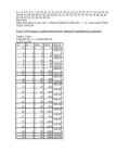
X5=5,01-6=-0,99 Y5=31,6*(-0,99)-47,483=-78,8 12. Fourier reaga sobitamise voimaluse analuus 1 1 1 1 1 t 0 1 2 3 4 5 6 7 8 9 0 1 12 3 4 5 8 2 1 9 3 2 2 1 3 8 4 x 0 5 0 4 6 6 8 7 7 74 0 5 12 3 7 5 Tabel 8. t x x*cost x*sint x*cos2t x*sin2t t c 3,5 0 5 5 0 5 0 4 0,23 6 4,5 3,96 0,75 5,95 4,5 0,45 25 3,9 24,69 -23,8 7,7 5 0,68 96 -51,4 81 -40,9 -86,9 5,5 0,9 80 -76 24,72 64,7 -47 5,7 75 -75 0 75 0
6,5 1,36 33 -14 -30 -21 25,4 7 1,59 27 7,54 -25,92 -22,8 -14,5 7,5 1,8 10 8,09 -5,87 3,09 -9,5 397 -222 58,67 64,04 -89,21 N=10 a0=x/n=397/10=39,7 a1=2*xcost/n=2*(-222)/10=-44,4 b1=2*xsint/n=2*58,67/10=11,73 a2=2*xcos2t/n=2*(64,04)/10=12,8 b2=2*xsin2t/n=2*(-89,21)/10=-17,8 Y1=a0+a1*cost+b1*sint y2=y1+a2*cos2t+b2*sin2t Y1,1=39,7-44,4*cos(0*180)+11,73sin(0*180)=-4,7 Y2,1=-4,7+12,8*cos(2*0)- 17,8*sin(2*0)=8,1 Y1,2=14,Y1,3=44, Y1,4=73, Y1,5=86, Y1,6=84 Y2,2=0, Y2,3=27, Y2,4=83, Y2,5=106, Y2,6=97
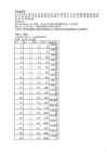
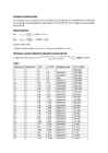
6.3 leitud normaaljaotuse tihedusfunktsioon f(x). Asetada modelleeritud arvud p.6.3 f(x) graafikule 𝑧𝑖 = ∑ 𝑃 − 6,00 𝑥𝑖 = 𝜎 ∙ 𝑧𝑖 + 𝑥𝑘 𝑥𝑖 1. -1.5 12.87 2. -1.16 21.63 3. -1.4 15.44 4. -0.57 36.85 5. 0.83 72.96 12. Analüüsida Fourier reaga sobitamise võimalust valimile t yi yi*cost yi*sint y1 yi*cos2t yi*sin2t y2 (yi-y1)^2 (y1-y2)^2 0 59 59 0 62.64664 59 0 64.38966 13.29797 29.04846 60 26 -25 -8 25.16142 21 15 57.02808 0.703213 962.742 120 71 58 41 71.66346 23 67 121.8109 0.440179 2581.747 180 76 -45 -61 20.57039 -22 73 70.3619 3072.442 31.78817
cos2 t cos t ja dx 2dt 1 cos tdt = = . x x2 + 2 2 2 tan 2 t cos2t cos t 2 sin2 t Viimase integraali leidmiseks teeme muutuja vahetuse z = sin t. Siis dz = cos tdt ja dx 1 dz 1 1 = 2 =- +C =- +C x2 x2 + 2 2 z 2z 2 sin t