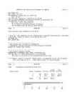
1.. T11 Te tootate 2.. T9 Teie vanus 3.. T10 Teie haridus Multiple R .49591 R Square .24593 Adjusted R Square .16792 Standard Error .79395 Analysis of Variance DF Sum of Squares Mean Square Regression 3 5.96197 1.98732 Residual 29 18.28046 .63036 F = 3.15268 Signif F = .0398 ------------------ Variables in the Equation ------------------ Variable B SE B Beta T Sig T T11 -.30526 .17483 -.33682 -1.746 .0914 T9 -.33646 .14191 -.39988 -2.371 .0246 T10 -.13837 .15698 -.17625 -.881 .3853 (Constant) 3.67551 .66999 5.486 .0000
Matemaatika ja statistika 2008/2009 SUMMARY OUTPUT Regression Statistics Multiple R 0,995 R Square 0,991 Adjusted R Square 0,991 Standard Error 0,063 Observations 180 ANOVA df SS MS F Signif F Regression 5 76,102 15,220 3811,568 1,02E-175 Residual 174 0,695 0,004 Total 179 76,797 Coefficients Std Error t Stat P-value Lower 95% Upper 95% Intercept -0,054 0,030 -1,811 0,072 -0,113 0,005 Inglise k 0,001 0,008 0,143 0,886 -0,015 0,018
calculate compensation values. • Provide precise inputs and hold the temperature during calibration. The results are only as good as the input value and the temperature control. The example just mentioned used a simple voltage monitor to illustrate the concept. In some systems, such as something that measures light or sound, providing precise inputs may be problematical. • If any components in the high-precision part of the circuit produce signif- icant self-heating, such as power dissipated in a resistor, the results will be less precise. This technique does not lend itself to large production volumes, due to the need to calibrate every system. And if the sensor is remote, temperature effects at the sensor cannot be compensated this way (but a second tempera- ture sensor mounted with the remote input sensor would permit such compensation). Noise and Grounding Figure 9